Aug 042023
 

How is this possible???? The 2023-2024 editions of Mexico’s free textbooks for school students are being roundly and rightly criticized on various fronts. Prepared and published by the Education Ministry (SEP), one of them includes this map:

v

Map in SEP textbook, 2023 edition

Time to play “Spot the Mistake.” Answer: Map has flipped the names of two states: Guanajuato and Querétaro. Astonishing! How is this possible?

Dear SEP: For future reference, Geo-Mexico is always happy to be contracted to provide proof reading and geography fact-checking…

And, if you thought the map was bad . . . at least it is almost correct, which is more than can be said for this graphic of the Solar System, taken from another 2023-2024 free SEP textbook:

We’re not going to insult the intelligence of our readers by pointing out why this is totally misleading!

To students and teachers everywhere: Have a happy and successful 2023-2024 Academic Year.

Feb 122017
 

One of the more beautiful, unusual and useful map projections ever devised was created by cartographer Bernard Cahill. The butterfly projection was first published in the Scottish Geographical Magazine in 1909. Cahill (1866-1944) later applied for a US patent to protect his creation.


I first came across Cahill’s projection on a stamp issued in Mexico in 1964. The design of the stamp (see image) shows his world map, an octahedral whose eight faces have been flattened into a shape resembling a butterfly. Ever since then I have wondered why such an unusual map would be chosen for a Mexican stamp that commemorated the 10th Conference of the International Bar Association (IBA), held that year in Mexico City. Coming some 20 years after the cartographer’s death, it seems an unlikely choice. So far, all my efforts to find a link between Cahill, the IBA and Mexico have drawn a blank. (Note to readers: Help needed!)

Cahill’s butterfly map, like Buckminster Fuller’s later Dymaxion Maps (1943 and 1954) enabled all the continents to appear linked, and with reasonable fidelity to a globe. Cahill demonstrated this principle by also inventing a rubber ball globe which could be placed under a pane of glass and flattened into the “Butterfly” form. When removed, the map/globe reverted to its original shape.

The original Cahill projection (1909). Credit: Gene Keyes

The original Cahill projection (1909). Credit: Gene Keyes

Largely in honor of his cartographic innovation, Cahill was elected a Fellow of the Royal Geographical Society. In 1913 he started the Cahill World Map Company, but this company was not successful and his map has since been largely forgotten by most people.

But not by cartographer Gene Keyes! Except for Cahill himself, no follower of Cahill’s projection has ever been as dedicated as Gene Keyes, a former student of Buckminster Fuller. Keyes’ website is a mine of information about Cahill and his map projection, and is well worth reading.

Born in the UK, Bernard Joseph Stanislaus Cahill (18661944) was an architect, town planner and cartographer who moved to San Francisco, California, in 1888. He was an early proponent of the San Francisco Civic Center and designed that city’s Neptune Society Columbarium.

Cahill encountered some stiff obstacles in the many years it took him to develop his butterfly projection. For example, he lost all his initial drawings and papers in the disastrous San Francisco earthquake and fire of 1906. At least one major publisher signed a contract to publish the butterfly map as a wall map and in an atlas, but then failed to follow through.

Cahill’s world map used for world tours

Soon after its creation, Cahill’s butterfly map was used to illustrate a flying trip around the world, or circumaviation, proposed for the Panama Pacific International Exposition held in San Francisco in 1915. The map was exhibited at this exposition and won a gold medal for cartography. Some time later, the map was used by both the State of California and the City of Charleston to illustrate shipping routes.

In 1924, the American Express Company chose the map for use during a world tour aboard the Cunard ocean liner Laconia. According to Keyes, the map was prominently displayed on the Palm Deck of the ship and seen by Robert Ripley, a participant on the world tour, who later featured it in his Believe it or Not series.

Perhaps the closest Cahill came to seeing his map in more general use came in 1937, when the International Meteorological Committee apparently came within a single vote of adopting a version of his projection for all world weather charting.

No wonder, then, that in Keyes’ words, “Cahill should be seen in company with other pioneers such as Charles Babbage or Gregor Mendel, who died long before their efforts gained wider appreciation. As well, he antedates Buckminster Fuller, prophet of Spaceship Earth.”

Keyes goes on to note that, “Cahill was not merely an astute architect and cartographer, but, that like Fuller, his map expressed an underlying whole-earth philosophy much like themes which emerged 60 years later. Cahill used the term “geosophy” in that regard….” (And used it as early as 1912, well before the geographer J.K. Wright, commonly credited for having coined the term in 1947).

Will Cahill’s map ever catch on? The latest sign of renewed interest in Cahill’s projection comes from its adaptation by the New York Times as the basis for a series of 10 maps published in December 2011 illustrating the changing world of computing, communications and technology.

Keyes closes his account of Cahill’s map by quoting Ambrose Bierce, who in a letter to Cahill, wrote that, “The Butterfly Map is indubitably the right one, but it will be a long time before it gets into general use….”

Sadly, that has proved to be all too true, despite its inclusion in the design of a Mexican postage stamp.

Related posts using Mexican stamps for illustration:

The geography of tequila: where is tequila made?

 Other  Comments Off on The geography of tequila: where is tequila made?
Nov 142016
 

The production of (genuine) tequila is tightly regulated because tequila has denomination of origin status. This status (sometimes called appellation of origin) sets specific standards for producers in terms of how a product is grown or produced, processed and presented. Equally importantly, it defines the geographic indication, the specific places or regions where the product has to be made. Other items having denomination of origin status include champagne, asiago cheese and Melton Mowbray pork pies.

Geographic indications are “indications which identify a good as originating in the territory of a Member, or a region or locality in that territory, where a given quality, reputation or other characteristic of the good is essentially attributable to its geographic origin.” (World Trade Organization)

Mexico’s denomination of origin area for genuine tequila includes includes 180 municipalities in five states, a total area of about 11 million hectares (27 million acres).

Tequila producing areas of Jalisco and neighboring states.

Tequila producing areas of Jalisco and neighboring states. Credit: Tony Burton; all rights reserved. Click to enlarge

The main area (see map above) is the state of Jalisco (all 124 municipalities), with extensions into three neighboring states:

  • Nayarit (8 municipalities): Ahuacatlán, Amatlán de Cañas, Ixtlán del Río, Jala, Xalisco, San Pedro Lagunillas, Santa María del Oro and Tepic.
  • Guanajuato (7 municipalities): Abasolo, Cd. Manuel Doblado, Cuerámaro, Huanimaro, Pénjamo, Purísima del Rincón and Romita.
  • Michoacán (30 municipalities): Briseñas de Matamoros, Chavinda, Chilchota, Churintzio, Cotija, Ecuandureo, Jacona, Jiquilpan, Maravatío, Marcos Castellanos, Nuevo Parangaricutiro, Numarán, Pajacuarán, Peribán, La Piedad, Régules, Los Reyes, Sahuayo, Tancítaro, Tangamandapio, Tangancicuaro, Tanhuato, Tinguindín, Tocumbo, Venustiano Carranza, Villa Mar, Vista Hermosa, Yurécuaro, Zamora, and Zináparo.
Tequila growing area in Tamaulipas.

Tequila growing area in Tamaulipas. Credit: Tony Burton; all rights reserved. Click to enlarge.

About 80% of all blue agave is grown in Jalisco, and almost all tequila distilleries are located in the state.

The municipality of Maravatío in the eastern section of Michoacán is a tequila outlier, some distance away from the main producing area centered on Jalisco.

The other major outlier is a group of 11 municipalities in the northern border state of Tamaulipas (see second map) where 11 municipalities (Aldama, Altamira, Antiguo Morelos, Gómez Farías, González, Llera, Mante, Nuevo Morelos, Ocampo, Tula and Xicotencatl) are included in the denomination of origin for tequila.

The first denomination of origin for tequila was registered with the World Intellectual Property Organization in 1978. Since that time every trade agreement signed by Mexico has contained a clause to ensure that tequila’s special status is fully protected by the other signatories. Mexico has signed free trade agreements with more countries than any other country in the world.

For example, the relevant NAFTA clause states that:

“Canada and the United States shall recognize Tequila and Mezcal as distinctive products of Mexico. Accordingly, Canada and the United States shall not permit the sale of any product as Tequila or Mezcal, unless it has been manufactured in Mexico in accordance with the laws and regulations of Mexico governing the manufacture of Tequila and Mezcal.”

In 1996, Mexico succeeded in getting the World Trade Organization to recognize tequila, and also mezcal, as denomination of origin products.

The following year, Mexico signed an agreement with the European Union whereby Mexico recognized 175 European spirits, including champagne, cognac, grappa and scotch, as having denomination of origin protection, in exchange for E.U. protection for tequila and mezcal. At that time, Mexico’s Tequila Regulatory Council (CRT) estimated that some 3.5 million liters of “pseudo-tequilas” were sold annually in Europe under such names as “Blue Tarantula” in Italy and “Hot Tequila” in Finland (In search of the blue agave: Tequla’s denomination of origin).

Related posts:

Alexander von Humboldt’s visit to Mexico, 1803-1804

 Other  Comments Off on Alexander von Humboldt’s visit to Mexico, 1803-1804
Sep 292016
 

Alexander von Humboldt‘s visit to Mexico began in Acapulco on March 22, 1803, and lasted for almost a year. (He left Mexico via Veracruz for the USA on March 7, 1804.) In his year in Mexico, Humboldt had been incredibly busy. He had measured, recorded, observed and written about anything and everything, with remarkable industry and accuracy. He had climbed mountains, burned his boots on active volcanoes, descended into mines, recorded geographical coordinates, and collected numerous specimens and antiquities. Humboldt’s Political Essay on the Kingdom of New Spain was the first systematic scientific description of the New World. It appeared in 1811, and marked the birth of modern geography in Mexico. His figures and ideas were used and quoted by writers for many many years.

Humboldt had also drawn a large number of maps, drawings and sketches and it can rightly be claimed that the modern era of Mexican map-making began with Alexander von Humboldt, and was then developed further later in the 19th century by cartographers such as Antonio García Cubas.

Humboldt's route in Mexico

Humboldt’s route in Mexico. Click to enlarge

Alexander von Humboldt (Self-portrait c1814)

Alexander von Humboldt (Self-portrait c1814)

The map above shows the route followed by Humboldt during his time in Mexico. The map comes from the book La obra de Alexander von Humboldt en México by Rayfred Lionel Stevens-Middleton  (Mexico D.F.: Instituto Panamericano de Geografía e Historía, 1956). This hard-to-find work is a comprehensive account of Humboldt’s time in Mexico and of his significance for the development of what the author refers to as “modern geography”.

The map of Humboldt’s route in Mexico includes his various side trips such as those to Jorullo Volcano and Santa María Regla.

Humboldt was keen to see Jorullo Volcano, since it was a rare example of a brand new volcano, one of only a handful of volcanoes that have emerged on land anywhere in the world in historic times. Jorullo first erupted on 29 September 1759 and activity continued for 15 years until 1774. Two centuries later, and about 80 km (50 miles) away, Paricutín Volcano burst into action for the first time, in a farmer’s field in 1943.

Santa María Regla, in the state of Hidalgo, about an hour’s drive north of Mexico City, is the best known location in Mexico for basalt columns. The columns, up to 40 meters tall,  are attractively located on the side of a canyon, with a waterfall tumbling over some of them:

Despite only seeing a relatively small part of the country (New Spain as it then was), Humboldt was able to make some generalizations about geography in general, and Mexican geography in particular, that have stood the test of time remarkably well. For example, he was the first to describe the vertical differentiation of climatic and vegetation zones in Mexico. Writing in 1811, he proposed the terms tierra caliente, tierra templada, and tierra fría, terms still widely used by non-specialists today:

Related posts:

Note: this post was first published on May 7, 2012.

Apr 282016
 

Like most geographers, I collect maps and information wherever I travel; you never know what surprises await. Tourism publications are especially interesting since they are specifically designed (one assumes) to show the best side of the places described.

My collection of tourist brochures associated with Jalisco and the Lake Chapala area dates back more than thirty years. Many early versions had stylized maps, drawn by graphic designers, not cartographers, with sound (if uninspiring) text in Spanish. English translations were often unintelligible. In the 1980s, several bilingual members of the now-defunct Association of Travel Reporters, based in Guadalajara, offered to help the Jalisco State Tourism Department improve its translations, but the offer was politely declined.

chapala-brochure-2016

As this latest brochure relating to Lake Chapala shows, translation standards have not improved significantly since then, and remain a long way off “native speaker” level. This is particularly unfortunate, given that this area of Mexico has the largest concentration of English-speakers in the country.

Here, for example, is the English translation of the attractions of San Juan Cosalá:

One has to closely experience San Juan Cosalá in order to feel and enjoy it to the most, so come and discover a place you will never want to leave, for every happy moment can be lived here, as just by visiting you feel enveloped in an affluent of joy and vitality.

In getting to know it, just stroll across its Pier, or admire the harmonious architecture in San Juan Evangelista Church, or enjoy the exquisite aromas of seafood, bouncing from restaurants enlivened with fine music while walking over the Piedra Barrenada (Drilled Stone); or the rest;  freshness and fun offered in thermal waterparks and world level spas.

Undated tourism brochure, collected April 2016

Undated tourism brochure, collected April 2016

The cartography (above) also leaves a lot to be desired. A key (not shown in this post) is provided but the Jalisco Tourism department clearly needs to hire a geographer if they want to publish useful and meaningful maps. Details worth noting include:

  • No symbol in the key for the “gas station” signs shown on the map. The map shows only four gas stations in this area (and none in Chapala or Ajijic); there are dozens of others not shown on the map, including several in Chapala and Ajijic.
  • The map has no scale.
  • The Isla de los Alacranes, a short boat-ride from Chapala, is shown a long way south of its true position, and a lot further from Chapala than it really is.
  • The dark blue area is, according to the key, the Chapala Lakeshore. I have absolutely no idea what it really represents! Lake Chapala’s catchment area is a completely different shape to the dark blue area. The “Chapala Lakeshore” should, obviously, also include the south-east section of the lake around Las Palmas and Cojumatlán. Much of the area colored dark blue is out of view of the lake, and drains towards the Santiago River, not the lake.
  • Placing the word “CHAPALA” in the north-east section of the dark blue area is totally misleading. The area where the word is written is NOT in the lake basin, not in view of the lake, and is not even in the municipality of Chapala. Again, I have no idea why the artist responsible for this map chose to ignore geography.

It is 2016, and Jalisco State tourism officials still need to improve the quality of their brochures and maps. Come on guys! Time to up your game!

Does Quintana Roo share a border with Guatemala? Not any longer.

 Maps, Updates to Geo-Mexico  Comments Off on Does Quintana Roo share a border with Guatemala? Not any longer.
Jan 072016
 

The state of Quintana Roo is Mexico’s youngest state (together with Baja California Sur), though this is set to change when Mexico City is formally declared a state, probably later this year. Quintana Roo, established in 1974, is well known to tourists because its largest city is the tourist mega-resort of Cancún, on Mexico’s Caribbean coast.

The northern part of Quintana Roo has a shoreline along the Gulf of Mexico. To the west of Quintana Roo lie the states of Yucatán and Campeche. But what about the southern limit of the state? Does it, or does it not, share a border with Guatemala?

In the early 1990s, the answer to this question was certainly “yes”, but things have changed since then, and the correct answer today is “not any longer”.

Boundary disputes in Yucatan Peninsula

  • Source: INEGI Map of the Disputed Areas

The state officially claims an area of 44,705 square kilometers (17,261 sq mi), but since 1996-97 there has  been a boundary dispute with the states of Yucatán and Campeche over an area of approximately 10,200 square kilometers (3,900 sq mi).

The contentious boundary issue arose when Campeche delimited a new municipality, Calakmul, in the south-east part of the state, and in doing so “annexed” a piece of Quintana Roo. This shifted the boundary between the two states towards the east, with a knock-on effect that the state of Yucatán also lost a small amount of territory to Campeche. However, Yucatán State simultaneously gained ground from Quintana Roo (see map). Confused? Well, that is really only the beginning, since the states of Yucatán and Campeche also dispute their shared boundary further north.

Confused administrative boundaries are never an easy thing to fix, and land boundary disputes are rife in Mexico at every level, so getting municipal, state and federal authorities to agree on a resolution takes time. The major Campeche-Quintana Roo dispute arose in the late 1990s, but was only finally settled, somewhat arbitrarily by federal court, in 2013. The court sided with Campeche, and Quintana Roo lost its border with Guatemala.

Oh dear… our Geo-Mexico map of Quintana Roo is now out of date!

Related posts:

Maps of Mexico on geo-mexico.com

 Index page, Maps  Comments Off on Maps of Mexico on geo-mexico.com
Dec 012015
 

This page lists some of the many maps on Geo-Mexico.com.

Want to use a map? All these maps [except those marked  (*)] are original Geo-Mexico.com maps. The use of any of Geo-Mexico’s maps for educational purposes is fine, provided credit is given to  Geo-Mexico.com. For commercial use (including business presentations, newsletters, magazines, books, TV), please contact us with details of your project via the link or the Contact Us form.

General / Educational:

Physical geography

Hazards:

Population

Economy

Regional and city maps

Crime:

History:

Other:

Mapping exercises:

 Tagged with:

The spatial development of Mexico’s railway network

 Excerpts from Geo-Mexico  Comments Off on The spatial development of Mexico’s railway network
Dec 202014
 

At the end of the nineteenth century, during the successive presidencies of Porfirio Díaz, railway building leapt forward. Díaz aggressively encouraged rail development through generous concessions and government subsidies to foreign investors. By 1884 Mexico had 12,000 km of track, including a US-financed link from Mexico City to the USA through Torreón, Chihuahua and Ciudad Juárez. A British company had completed lines from Mexico City to Guadalajara, and from Mexico City via Monterrey to Nuevo Laredo.

Fig. 17.2 The development of Mexico's railway network

Fig. 17.2 The development of Mexico’s railway network. Copyright: Geo-Mexico; all rights reserved

By the start of the twentieth century, additional tracks connected Guadalajara, San Luis Potosí and Monterrey to the Gulf coast port of Tampico. A line connecting the Pacific and Gulf coasts was also completed. Durango was now connected to Eagle Pass on the US border. A second line to Veracruz was constructed, with a spur to Oaxaca. Laws passed in 1898 sought to bring order to the rapid and chaotic expansion of Mexico’s rail system. Foreign concessions were restricted. Subsidies were only made available for the completion of missing links such as lines to Manzanillo and the Guatemala border. Efforts were made to standardize track gauges.

After the Revolution, network improvements were hindered by poor administration, corruption, labor unions and a shift of government priority to roads. The west coast railroad from Sonora to Guadalajara was completed in 1927. The Yucatán Peninsula was joined to the national network in the 1950s and the famous Chihuahua to Los Mochis line through the Copper Canyon was completed in 1961, finally linking Texas and Mexico’s northern plateau to the Pacific Ocean.

Related posts:

Where are Mexico’s mangrove swamps?

 Updates to Geo-Mexico  Comments Off on Where are Mexico’s mangrove swamps?
Aug 142014
 

The National Commission for the Knowledge and Use of Biodiversity (Comisión Nacional para el Conocimiento y Uso de la Biodiversidad, CONABIO), has identified 81 distinct areas in Mexico that have mangroves with “biological significance and in need of varying degrees of ecological rehabilitation” (see summary map). These regions are distributed as follows:

  • 10 on the northern Pacific Coast
  • 6 on the central Pacific Coast
  • 13 on the southern Pacific Coast
  • 27 on the Gulf of Mexico and
  • 25 on the Yucatán Peninsula.

A national inventory has now been compiled by CONABIO. All areas have been surveyed and preliminary descriptions published including details of their location, size, physical characteristics, socioeconomic conditions, local uses of mangrove, biological details, including vegetation structure, and an assessment of local impacts and risks, management and existing conservation measures.

Map of distribution of mangroves in MexicoThe areas of mangroves have been mapped at a scale of 1:50,000 and satellite photos from 2005-2006 have been used in conjunction with fieldwork to calculate the areas of mangroves. The final map is believed to be more than 90% accurate, a reasonable baseline for future comparisons. CONABIO is planning to resurvey the mangrove areas every 5 years following the same methodology.

According to preliminary comparisons with previous attempts to quantify the extent of mangroves in Mexico (the subject of a future post), the loss of mangroves was greatest in the period 1970-1980, and in 2000-2005, but then diminished in the period 2005-2010.

Between 2005 and 2010, the states where mangrove loss remained high (as a percentage of the total area of mangroves in the state) included Chiapas, Baja Californa Sur and Sonora. However, the states losing the largest areas of mangroves in absolute terms were Quintana Roo, Campeche and Nayarit. Jalisco has the unfortunate distinction of being the state where coastal mangrove loss was highest (in terms of the proportion of its total coastline length bordered by mangroves).

Related posts:

The regional geography of tacos

 Books and resources  Comments Off on The regional geography of tacos
Jun 072014
 

A taco is a corn or wheat tortilla folded or rolled around other edible ingredients, and designed to be eaten by hand – the indigenous Mexican equivalent of a sandwich. Tacos are extremely versatile and often accompanied by garnishes such as tomatoes, onions, lettuce, radishes, and avocado or guacamole, topped with salsa and cilantro.

Who would have thought that the humble taco was worth its own encyclopaedia? This particular encyclopaedia includes a fascinating graphic – a map (see graphic) summarizing the different regional varieties of taco commonly found in different parts of the country.

The accompanying terminology used to describe all these tacos is mind-blowing, but a small sampling will give you the idea:

Regional varieties of Mexican tacos

Regional varieties of Mexican tacos. Credit: La tacopedia. Enciclopedia del taco (Spanish Edition) . Click to enlarge.

The map is by no means an exhaustive list, but does include examples of taco specialties for every state.

The two states occupying the Baja California Peninsula both have seafood-based tacos:

  • Baja California – tacos de langosta con frijoles (lobster and beans tacos)
  • Baja California Sur – tacos de marlin ahumado (smoked marlin tacos)

The tacos popular in some states reveal less about their ingredients:

  • Aguascalientes – tacos mineros (miner’s tacos)
  • Coahuila – tacos laguneros (Laguna region tacos)
  • Morelos – tacos acorazados (battleship tacos)
  • Puebla – taquitos miniatura (miniature tacos)

For some unusual ingredients, try:

  • Chiapas – tacos de hormiga chicatana (flying ant tacos)
  • Colima – tacos de sesos (brain tacos)
  • Hidalgo – tacos de gusanos de maguey (maguey worm tacos)
  • Yucatán – tacos de tzic de venado (shredded venison tacos)

Feeling daring? Try the tacos envenenados in Zacatecas. The literal meaning is “poisoned tacos”, but they are apparently named so as not to reveal all their ingredients!

Tacos have become incredibly popular. While they predate the Spanish conquest, they are now well on their way to conquering large swathes of North America and Europe.

The regional patterns is analyzed further by Frank Jacobs in 604 – A Tacography of Mexico

For more about tacos, we recommend reading La tacopedia. Enciclopedia del taco by Deborah Holtz and Juan Carlos Mena (Trilce Ediciones, 2012).

Related posts:

The pattern of farm sizes in Mexico: is there a north-south divide?

 Other  Comments Off on The pattern of farm sizes in Mexico: is there a north-south divide?
Feb 242014
 

In 2007, INEGI census recorded 2.4 million “units of production” (farms) under 2 hectares in size. This number is 43.5% of all farms, and includes farms not being actively worked. 22.9% of farms were between 2 and 5 hectares in area and a further 23.4% between 5 and 20 hectares. In sum, almost 90% of all farms had an area of 20 hectares or less. At the other end of the size spectrum, 2.2% of farms were larger than 100 hectares.

In terms of land tenure, 68.5% of all farms were in ejidos (a form of collective farming), 28.5% held privately and the remaining 3% were other (communal, public, mixed). Almost three-quarters of all farms under 20 hectares in area are ejidos, whereas about three-quarters of all farms over 100 hectares in size are private.

Map of average farm size in Mexico, by state, 2007

Map of average farm size in Mexico, by state, 2007. Data: INEGI. Credit: Tony Burton/Geo-Mexico

The choropleth map (above) shows the average size of farms (in hectares) by state. It is very clear that larger farms are concentrated in northern Mexico. All the states along the US border have average farm sizes in excess of 100 hectares. At the other extreme, a ring of states in central Mexico (centered on the Federal District) have average farm sizes that are below 5 hectares. The average farm size is slightly larger to the south of that ring of tiny farms, and significantly larger towards the east, including those states comprising the Yucatán Peninsula.

The general pattern is of a north-south division, which becomes even clearer when the average farm sizes are plotted as an isoline map. With minor exceptions, the “surface” represented by these isolines slopes steeply away form the highest values in north-western Mexico towards the south-east.

Average farm size in Mexico

Average farm size in Mexico. Data: INEGI Credit: Tony Burton / Geo-Mexico

Classroom exercise

Having recognized this pattern in farm sizes, can you think of reasons that might explain it? The short answer is that farm sizes vary in response to a multitude of factors, These include historical, demographic, and socioeconomic factors as well as relief, climate, natural vegetation and soils.

Q1. Compare the maps in this post with maps for some of the factors you think might be important. (Try our Geo-Mexico Map Index as a starting point). For example, the northern area of Mexico, the area with largest farms, is primarily semi-arid or arid. Why might farms in arid and semi-arid areas be larger than in other areas?

Q2. Have a class discussion about the relative importance of the factors that have been identified or suggested.

Q3. Discuss the relative merits of the two mapping methods used in this post (choropleth and isoline) to portray average farm sizes.

Related posts:

Geo-Mexico has many other agriculture-related posts (easily found via our tag system). They include posts about the geography of growing/producing Christmas trees, cacao, honey, sugarcane, coffee, chiles, floriculture, tomatoes, tequila, horticultural cropsand oranges. Also worth reading are:

The pattern of violent crimes in Mexico in 2013

 Mexico's geography in the Press, Updates to Geo-Mexico  Comments Off on The pattern of violent crimes in Mexico in 2013
Feb 082014
 

The Consejo Ciudadano para la Seguridad Pública y la Justicia Penal AC, a Mexican non-profit, has published an interesting report looking at the levels of violent crime in Mexico in 2013:

The authors take violent crimes to include intentional homicide, kidnapping, rape, aggravated assault, robbery with violence and extortion.

At the municipal level, violent crime is concentrated in a relatively small number of municipalities. The report looks at the statistics for the 216 municipalities (including delegaciones of the Federal District) that had estimated populations of over 100,000 in 2013. Since 2012, four municipalities have joined this group: El Fuerte (Sinaloa), Tepotzotlán (México), Pánuco (Veracruz) y Playas de Rosarito (Baja California). Between them, the 216 municipalities are home to about 64% of Mexico’s total population.

Data from government agencies and INEGI were used to compile rates for each crime in each municipality. These rates were then multiplied by the following weightings (to reflect the relative severity and impacts of each type of crime),

  • 0.55 for intentional homicide
  • 0.22 for kidnapping
  • 0.13 for rape
  • 0.04 for aggravated assault
  • 0.03 for robbery with violence
  • 0.03 for extortion

and summed to give an overall index for “violent crimes”.  For the 231 municipalities, the index ranged from 106.63 for Oaxaca, Oaxaca to 0.00 for Zapotlán el Grande in Jalisco. The full details of the methodology are explained and discussed in the report. A similar methodology was also used to calculate levels of violence by state.

The worst 10 municipalities in terms of violent crime were:

  1. Oaxaca, Oaxaca – violent crime index value of 106.63
  2. Acapulco, Guerrero – 80.35
  3. Cuernavaca, Morelos – 65.30
  4. Yautepec, Morelos – 56.19
  5. San Pedro, Coahuila – 53.42
  6. Cd. Victoria, Tamaulipas – 52.48
  7. Iguala de la Independencia, Guerrero – 52.25
  8. El Fuerte, Sinaloa – 50.82
  9. Jiutepec, Morelos – 50.29
  10. Torreón, Coahuila – 49.31

The national index (ie treating the entire country as a single entity) was 23.17, meaning that the index value for violent crimes in Oaxaca, Oaxaca, was more than four times that of the country as a whole.

Municipalities which were in the worst twenty in 2012 for violent crime, but have now fallen out of that group include: Lerdo (Durango) Zacatecas (Zacatecas), Cuautla (Morelos), Zihuatanejo (Guerrero), Temixco (Morelos), Cuauhtémoc (DF), Tecomán (Colima), Navolato (Sinaloa), Centro (Tabasco) and Monterrey (Nuevo León).

Moving into the worst twenty for the first time are: Playas de Rosarito (Baja California), Hidalgo del Parral (Chihuahua) San Pedro (Coahuila), Chilpancingo (Guerrero), El Fuerte (Sinaloa) and Chalco, Cuautitlán, Cuautitlán Izcalli, Ecatepec and Naucalpan (all in the State of Mexico).

Of the 213 municipalities, Acapulco had the highest intentional homicide rate (112.81/100,000, about 6 times the national rate of 19.05/100,000). Cd Victoria had the highest kidnapping rate (23.28/100,000, 15 times higher than the national rate of 1.46/100,000, though kidnapping rates in Mexico are notoriously unreliable, and have been the subject of intense press debate in recent months).

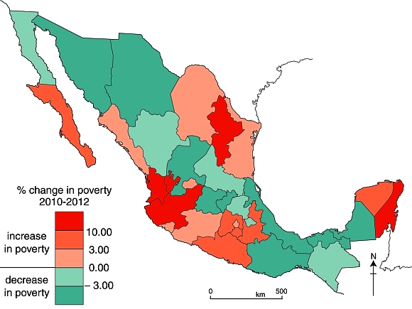
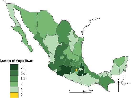
Violent crimes by state, 2013

By state (see map), Guerrero had the highest violent crime index with 47.76 points, followed by Morelos 43.99 and Chihuahua 40.87. In general, with the prominent exceptions of the State of México and Guerrero, the southern half of Mexico appears to be somewhat safer than the northern half.

Map of Violent crime index, 2013

Violent crime index, 2013. Source of data: see post. Credit: Geo-Mexico

For individual categories of crime at the state scale, Morelos had the highest kidnapping rate (8.24/100,000). Quintana Roo had the highest rate of rape (28.31/100,000, compared to national average of 11.36/100,000). The State of Mexico had the highest rate for aggravated assault (251.64/100,000 compared to national average of 130.21/100,000). Morelos came out on top for the highest rate of robbery with violence (455.08/100,000 compared to national average of 182.61) and for the highest rate of extortion (21.96/100,000 compared to national average of 6.94/100,000).

Good news for tourists

According to this report, almost all of Mexico’s major tourist destinations (with the noteworthy exception of Acapulco) are located in areas where violent crime is below the national average.

Related posts:
Jan 022014
 

The total number of people living in poverty in Mexico continues to rise, though the poverty rate (as a percentage) remains roughly the same. According to Mexico’s National Political and Social Development Commission (Spanish language acronym: Coneval), the number of people in poverty has risen steadily for several years, much in line with Mexico’s rising total population. Coneval’s figures are based on a simple multidimensional poverty index, which considers the following criteria:

  • household income
  • access to education
  • access to food
  • access to health care
  • access to social services
  • housing quality
  • access to basic household services (electricity, water, drainage)

According to Coneval, 53.3 million Mexicans (45.5% of the total population) were living in poverty in 2012, compared to 52.8 million (46.1% of the then population) in 2010 and 48.8 million Mexicans (44.5%of the population) in 2008.

Note that poverty statistics prior to 2008 in Mexico were generally based purely on income levels. From 2008, this method was replaced by a multidimensional index. The precise details of the index have been modified slightly since that time, making exact comparisons between 2012 and 2008 more problematic.

While the precise numbers are subject to debate, mainly due to differing definitions of what constitutes “poverty” and how it can be measured, the trend revealed by the Coneval numbers is supported by the Economic Commission for Latin America and the Caribbean (ECLAC) in its “Social Panorama of Latin America 2013“, published in December 2013. The ECLAC report found that Mexico is one of a very few countries where poverty levels rose between 2011 and 2012, from 36.3% of the population to 37.1%, according to its definition.

The dire situation in Mexico compares to a slight decrease in poverty in most larger Latin American countries, including Venezuela, Ecuador, Brazil, Peru, Argentina and Colombia.

In absolute terms, according to ECLAC, 164 million people were found to be living in poverty in Latin America, about 57.4 million (35%) of them in Mexico.

Change in poverty rates in Mexico, 2010-2012.

Change in poverty rates in Mexico, 2010-2012. Credit: Geo-Mexico; all rights reserved. Data: Coneval

The map shows the Coneval data for changes in the poverty rate between 2010 and 2012 by state. It appears that poverty levels increased in many of Mexico’s more prosperous areas and in the longer established industrial areas, as well as in almost all areas where tourism is important. Poverty decreased in some of Mexico’s more rural, and generally poorer, states.

Related posts:

Example of a sixteenth century map

 Other  Comments Off on Example of a sixteenth century map
Dec 072013
 

In the mid-sixteenth century, the Spanish Court was determined to acquire accurate information about everything being encountered in New Spain. This led to a series of censuses and accounts, including the Relaciones geográficas (Geographic Accounts).

The basis for the Geographic Accounts was a 50-question survey, sent to New Spain in 1577. The authorities in each administrative center were instructed to call a meeting of the “Spaniards and other natives in the district”, to find out everything they could about the area’s geography, people and history.

Of the 191 known responses to the 1577 questionnaire, 167 have survived in archives to the present day. Most of the original responses are housed in Spain, in either the Archivo General de las Indias in Seville or the Real Academia de la Historia in Madrid, while a further 43 responses form part of the Benson Latin American Collection in the University of Texas library in Austin. (The library’s webpage about the Relaciones geográficas has several links to images of sample pages and maps).

Map of Zempoala area from the Relaciones Geográficas

Map of Zempoala area from the Relaciones Geográficas (1577)

The accounts contain a wealth of information about population, relief, flora, fauna, economic activities and lifestyles. Some also include maps of the areas being described. However these early maps do not follow modern conventions in terms of having a uniform scale across the area being shown, or an orientation that is consistent in terms of compass directions. They are pictorial maps, where the scale varies across the map, and where areas are delimited, or places are linked, without apparent regard for direction.

One such map (see image above) depicts the area around Zempoala (Hidalgo). This is analyzed by Barbara E. Mundy, Associate Professor of Art History at Fordham University, in an online article, Mapping Babel: A Sixteenth-Century Indigenous Map from Mexico, published in The Appendix, a “journal of narrative and experimental history”. In the article, Mundy provides a detailed, step-by-step account of the map, with lots of additional related images and information.

Detail of map, showing Tepemayalco

Detail of map, showing Tepemaxalco

Mundy’s analysis reveals several “acts of translation” that have been made by the indigenous artist(s) presumed to be responsible for drawing the map.

For example, the artist(s) made the Spanish paper provided for the map more closely resemble its indigenous counterpart (bark paper), by joining sheets together to create the size they wanted for the map. In addition, unlike modern maps where the viewer is essentially static, with the map details arranged around them, indigenous maps demand changes of perspective, mobile viewers, who have to reorientate themselves depending where they are on the map in order to see things clearly.

Many of the images are a translation, perhaps of similar European images. For instance, like most towns on the map, Tepemaxalco is shown with “a conventional sign for a Christian chapel: a small building drawn in perspective with one side marked by a shadowing grey wash, topped with belfry and cross.”

The map also links the pictograph for each place name to its name written in alphabetic script. “The pictograph for Tepemaxalco (see image) registers some of its Nahuatl components: tepetl, ‘hill,’ maitl, ‘hand,’ xalli, ‘sand’ and co, ‘place of.’ Below, the name is written in alphabetic script, probably introduced by the Franciscans who evangelized this region.”

The dominant pictogram on this map is that for Zempoala (written “Cenpoballa” on the map). Mundy offers an interesting interpretation of this pictograph, which we hope to examine further in a future post.

Further reading

Barbara E Mundy. 2001. The Mapping of New Spain: Indigenous Cartography and the Maps of the Relaciones Geográficas.

Related posts:

Nov 162013
 

In an alliance with the Sonoran Institute, the National Geographic Center for Sustainable Destinations helped the region’s communities create the first transborder Geotourism MapGuide, covering northern Sonora and southern Arizona. The mapguide was published in 2007:

The maps  have vignettes of information about history, culture, geology and many other aspects of the region, making it a useful guide for geo-tourists. While some might argue about the choice of locations and attractions described on the maps, this is a useful addition to the background reading for anyone thinking of traveling to this region with some time on their hands to explore.

Surprisingly, the map has only a very brief and somewhat dismissive mention of the El Pinacate and Gran Desierto de  Altar Biosphere Reserve:

“Stand at the rim of this mile-wide volcanic crater and you may feel as if you’re on the moon. This land of ancient lava, sand, and cinder cones is sacred to the O’Odham people. Today, those on the Sonora side of the border call themselves “Pápago.”

Related posts:

The growth of the city of Monterrey, Mexico’s industrial powerhouse

 Excerpts from Geo-Mexico, Other  Comments Off on The growth of the city of Monterrey, Mexico’s industrial powerhouse
Oct 282013
 

A series of historical maps of the city of Monterrey was published earlier this year in the city’s online Catalog of Buildings of Historic and Artistic Importance in Barro Antiguo, The maps, dated 1765, 1791, 1846, 1865, 1922, 1933 and 1947 respectively, offer a good basis for considering the urban growth of Monterrey, the industrial powerhouse of northern Mexico.

In chapter 22 of Geo-Mexico, the geography and dynamics of modern Mexico, we explained why, “Monterrey does not fit the general Latin American urban model as well as Mexico City or Guadalajara. First, it never really existed as a colonial city. Secondly, its development was more heavily dependent on industry. Thirdly, its relative wealth and progressive leadership in some ways make it more similar to a North American city than a Latin American city. It fits the model only in that it developed a definite high status sector in contrast to lower status industrial sectors, and eventually became spatially fragmented.”

But just how did Monterrey develop as a city? In each of the following historical maps of Monterrey, Barrio Antiguo (16 blocks in size in the present-day city) is marked by a red quarter-circle, which is an easy way to check each map’s orientation and scale. Monterrey was founded in 1596. The earliest map in our series, for 1765, shows that, even by that date, Monterrey was still a relatively small settlement situated between a (seasonally dry) “stream formed by various springs” (to the top of the map, north) and the seasonally-dry “Monterrey River” (now called the Santa Catarina River). The Barrio Antiguo is shown as mostly an empty area, with only one major construction.

Monterrey 1765

Monterrey 1765

Very little has changed by 1791 (see map below: note that this map is oriented south-upwards), though the Barrio Antiguo has now been developed, and is shows as having several streets in a clear grid pattern:

monterrey-1791

Monterrey in 1791

The grid pattern for Barrio Antiguo is equally evident in the details of the map in 1846:

monterrey-1846

Monterrey in 1846

As of 1846, no development is shown on the south bank of the Santa Catarina River, though tracks are shown heading east and south-east respectively from the city. The next map, for 1865, shows that the city is beginning to expand to the south. A substantial settlement is developing on the south bank, more of less opposite the Barrio Antiguo. Note, though, that this map shows only part of the city:

monterrey-1865

Monterrey in 1865

Clearly, Monterrey only emerged as a real city after the colonial period which ended in 1821. The relatively small city did not experience real growth until late in the 19th century when it became connected by railroad and started to attract industrial development.

Early in the 20th century, investors built the then largest iron and steel works in Latin America a few kilometers east of the city center. Many related industries located nearby. These industries and the railroad, which ran east–west about four kilometers (2.5 mi) north of the city center, stimulated early industrial development in these directions. Developers established low income housing tracts for industrial and other workers on the east, north and west periphery of the city. Neighborhoods for the wealthier classes were developed south of the city center.

By 1933, Monterrey has grown significantly in area, especially towards the north:

monterrey-1933-whole-city

The city of Monterrey in 1933

Between 1933 and 1947, the city continues to expand, with many areas being infilled with residences:

monterrey-1947

The city of Monterrey in 1947

The city experienced another surge of industrialization and immigration in the 1950s and 1960s. Industrial development continued after 1970 when the national government implemented policies to shift development away from Mexico City. Monterrey became a major producer of steel, metal fabrication, cement, beverages, petrochemicals, food, telecommunications, auto parts, glass, and house furnishings. It also developed into a major financial center and one of the wealthiest and most progressive cities in the country.

Low income housing became a serious problem after the 1960s as the inner city tenements became extremely crowded. The government was not sympathetic to irregular housing schemes, so low income groups established numerous illegal squatter settlements on vacant land near the industrial zone. Government made a few efforts to remove these, but most survived and eventually became regularized.

The high status sector expanded south-west into San Pedro Garza García, which became one of the wealthiest municipalities in Mexico. The high overall income and wages in the city meant that many workers could afford home ownership and private automobiles. As a result, many gated communities (large and small) and suburban shopping malls were built around the urban periphery. The urban area became relatively fragmented with many low income residential zones located near high income areas.

Source of the maps used in this post:

Other posts about the urban geography of Mexico’s cities:

The pattern of homicides in Mexico in 2012

 Mexico's geography in the Press  Comments Off on The pattern of homicides in Mexico in 2012
Aug 172013
 

Homicide rates in Mexico increased between 2010 and 2012, though there is some evidence that they are now beginning to fall again. Did the pattern of homicide rates also change since 2010?

The top map shows the pattern of intentional homicides in Mexico in 2010. As we commented at the time, this map shows “that many northern states like Chihuahua, Sinaloa, Nuevo León and Durango are plagued by drug war violence and have very high murder rates. On the other hand, most states in the south and southeast, like Yucatán, Campeche and Tlaxcala are relatively free of drug war violence and historically have had low murder rates. One significant anomaly in the overall pattern appears to be Guerrero which is well to the south but has a high murder rate and a very significant amount of drug violence.”

Map of intentional homicide rate, 2010

Map of intentional homicide (murder) rate, 2010 Credit: Tony Burton / Geo-Mexico

The second map shows the pattern of intentional homicides in Mexico in 2012. (Note that the values on the key are slightly different to reflect the increase in Mexico’s average (nationwide) homicide rate between 2010 and 2012).

Map of homicide rates in Mexico, 2012, Credit: Tony Burton/ Geo-Mexico

Map of intentional homicide (murder) rates in Mexico. Credit: Tony Burton/ Geo-Mexico

At first sight the pattern in 2012 look pretty similar to that for 2010. The adjoining states of Sinaloa, Chihuahua and Durango continue to have rates well above the national average, as does Guerrero further south. However, the homicide rate in Nuevo León, which was “well above average” in 2010 has declined somewhat to “above average” in 2012. Since 2010, the north-eastern state of Tamaulipas has seen its homicide rate increase from “above average” to “well above average”. Perhaps more significantly, the border state of Coahuila has witnessed a jump from “below average” to “well above average”. Homicide rates in the two north-west border states of Baja California and Sonora have fallen since 2010 to “below average”.

Elsewhere, homicide rates have increased in both Zacatecas and in Colima since 2010, while rates in Veracruz have declined to “below average”. The shift in Veracruz means that a broad swathe of southern Mexico, including the Yucatán Peninsula, Oaxaca and Chiapas, now has a homicide rate “below average” or “well below average”, good news for tourists headed for Oaxaca, Cancún and the Riviera Maya!

On a more cautionary note, the state of Michoacán has seen increased violence in 2013; its homicide rate is headed upwards.

The changes in pattern of homicides between 2010 and 2012 are partially attributable to the “zones of contention” between rival drug gangs. For instance, the Knights Templar cartel (currently thought to be Mexico’s third largest cartel, behind the Zetas and the Sinaloa cartel) has its origin in  Michoacán but has expanded its geographic influence very rapidly in the past few years. Equally, the capture of key cartel leaders in recent years seems to herald increased violence as rivals compete to fill the perceived power vacuum left behind. This unfortunate outcome from the arrest of leading cartel operatives is continuing this year following the capture of Zeta leader Z-40.

Related posts:

Mexico’s seven climate regions

 Excerpts from Geo-Mexico  Comments Off on Mexico’s seven climate regions
Aug 152013
 

Climatologists have developed several scientific systems to classify climates. The system developed by Wladimir Köppen in the early 20th century is one of the earliest and best known. The Köppen climate classification system assumes that climate is best reflected in native vegetation and can be accurately classified using seasonal variations in temperatures and precipitation. Mexican climatologists, including Enriqueta García, have proposed minor modifications to the Köppen system to make it more appropriate for Mexico. The following paragraphs reflect García’s revised Köppen system.

Given that Mexico has many mountains with rapid changes in elevation, temperature and rainfall, applying the Köppen system, even as modified by García, to Mexico can become extremely complicated. A relatively small area of Mexico may include several Köppen climate categories. Aggregating these areas provides a less complicated, more understandable, picture of Mexico’s climates (see map). In this scheme, Mexico has seven main climate regions, as shown on the map:

Major climate regions in Mexico. (Fig 4-5 of Geo-Mexico, the geography and dynamics of modern Mexico). All rights reserved.

Major climate regions in Mexico. (Fig 4-5 of Geo-Mexico, the geography and dynamics of modern Mexico). All rights reserved.

Two tropical climates

Mexico has two tropical climates which have average temperatures of over 18°C (64°F) for all twelve months of the year.

The first, tropical wet (Af in the Köppen system, see map), has at least 60 mm (2.4 in) of rain in every month of the year. This is the climate of the Amazon and Indonesian rainforests. In Mexico this is the climate of the Gulf Coast Plain in southern Veracruz and Tabasco (classic tierra caliente areas). It also occurs in the Oaxaca and Chiapas highlands. The rains fall all year, varying from about 120–150 mm (4–5 in) in April to 380 mm (15 in) in September.

The tropical wet-and-dry (Aw) category (see the climate graph for Cancún) has a pronounced dry season. The dry winter months typically get less than 40 mm (1 in) of rain, compared to over 150 mm (6 in) in each of the summer months. Parts of West Africa, Brazil and India have a similar climate. Much of coastal Mexico, stretching from Nayarit along the Pacific coast all the way to Guatemala, is in this category. It also covers many inland areas along the Pacific coast. Central and northern Veracruz and most of the Yucatán Peninsula also have this tropical climate with summer rains.

Climate graphs for three cities. (Fig 4.6 of Geo-Mexico,)

Climate graphs for three cities. (Fig 4.6 of Geo-Mexico, the geography and dynamics of modern Mexico) All rights reserved.

Two dry climates

Areas with an arid (desert) climate (BW) usually receive less than 250 mm (10 in) of rain a year (see climate graph for Ciudad Juárez). This is the climate of the Sahara Desert and Central Australia. In Mexico dry desert areas include most of Baja California, western Sonora, and the northern section of the Central Plateau. These areas can experience frost and freezing during the winter.

Areas with the second type of arid climate, semiarid (dry steppe) (BS), receive 250–750 mm (10–30 in) of rain a year. This is the climate of the African savanna lands and much of central Asia. In Mexico, this climate region includes most of the Central Plateau as well as western sections of the Western Sierra Madre, northern Yucatán and scattered inland areas as far south as Oaxaca. The rains in this region fall mostly in the summer, and localized heavy thunderstorms are quite common. The southern parts of this climatic region are warmer than the northern parts.

Three temperate zones

Temperate climates typically have average temperatures above 10°C (50°F) in their warmest months, and a coldest month average between 3°C and 18°C (27–64°F). Moisture characteristics distinguish between the three temperate climates.

The temperate with dry winters climate (Cw) is characterized by mild temperatures, low humidity, and summer rainfall ranging from about 600 to 1200 mm (25–45 in) per year (see climate graph for Guadalajara). This is classic tierra templada country. The low nighttime temperatures in winter are typically around 5°C (41°F). Of course, higher elevations have lower temperatures with occasional frost. The highest temperatures usually reach about 35°C (95°F), though temperatures may reach as high as 40°C (104°F). This climate is similar to that of the Kenyan Highlands. In Mexico, this climate includes parts of Nuevo León and Tamaulipas, most of the Western Sierra Madre and many mountainous areas in western, central and southern Mexico. Most of the Volcanic Axis is in this temperate with dry winters zone. Here, the major control as far as temperatures are concerned is altitude, which directly affects precise rainfall amounts and seasonality, resulting in a mosaic of microclimates and natural vegetation regions.

Compared with the temperate with dry winters climate, the humid subtropical (Cf) zone gets more rainfall, is more humid and gets rain throughout the year. The only areas of Mexico with this climate are the eastern slopes of the Eastern Sierra Madre and some parts of the southern mountain systems.

The Mediterranean climate (Cs) is the mild climate associated with Europe’s Mediterranean coast as well as the California coast. The area around Tijuana is the only part of Mexico with this type of climate. This area is relatively arid and gets less than 400 mm (15 in) of rain a year; it is unique in Mexico, being the only place that is dry in summer and gets rain only in winter.

Related posts

Jul 242013
 

The map below shows a regional division of Mexico by precipitation regime (the amount and seasonal distribution of precipitation). The small graph for each region shows the typical average precipitation amounts for each month of the year. (For example, region A has most precipitation in the first three or four months of the year, and very little after that). The map comes from Ernesto Jáuregai’s 1970 article about wind and water erosion in Mexico (full reference is given below).

Precipitation regimes in Mexico (Fig 2 of Jáuregai 1970)

Precipitation regimes in Mexico (Fig 2 of Jáuregai 1970)

It is clear from the map that the distribution of precipitation across Mexico is very uneven. In general the north and central plateaus are dry while the southeast receives by far the most rain. Parts of Tabasco, Northern Chiapas and Veracruz get over 4000 mm (160 in) of rain a year. This is a direct effect of the onshore north-east trade winds, which collect moisture as they cross the Gulf of Mexico and then deposit it as they reach land.

Average annual rainfall figures conceal great differences from one year to the next. In general, the variability of rainfall is indirectly proportional to the long-term average. This means that areas with low totals tend to experience high variability, greatly increasing their drought hazard.

The map also reveals that there is a marked seasonality to precipitation in almost all of Mexico, with a clear division into a wet and a dry season. Most places get almost all their rain between June and October, while January through May are dry months. Because most rainfall is in the summer months, about 71% of rainfall evaporates soon after falling. This figure can be even higher in urban areas. Only about 26% runs off into rivers and lakes, and 3% seeps down to recharge subterranean aquifers.

One apparent anomaly to the pattern shown on the map is that the extreme north-west corner of Baja California (region A) has a Mediterranean climate where summers are dry and most rain falls in winter. Elsewhere in Mexico winter months are relatively dry. Southern and central Mexico have markedly dry winters, receiving less than 5% of their annual precipitation totals in the first three months of the year. The northern half of Mexico and the eastern coastal strip, including the Yucatán peninsula, have slightly more balanced precipitation, receiving between 5 and 18% of annual totals between January and March.

Map reference:

Ernesto Jáuregai. 1970. “La erosión hidráulica y eólica en México y sus efectos en las estructuras hidráulicas y en los núcleos de población.” UNAM: Boletín del Instituto de Geografía, Vol III, pp 39-60.

 Related posts

The three main causes of precipitation in Mexico

 Excerpts from Geo-Mexico  Comments Off on The three main causes of precipitation in Mexico
Jul 222013
 

The three basic types of rainfall (convectional, orographic and cyclonic) all play a role in determining the amount and timing of precipitation in Mexico.

Why does it rain?

In Mexico, most precipitation falls as rain, though snowfalls are not uncommon in parts of northern Mexico or at the highest elevations where air temperatures are cooler. For precipitation to occur, the air must first acquire moisture. Warm air absorbs water through evaporation from nearby bodies of water and through evapotranspiration from plants. The amount of water the air holds compared to the maximum amount it can hold at that temperature is the relative humidity. If warm moist air rises, it will cool. As it cools, its relative humidity rises. If relative humidity reaches 100% and condensation nuclei (particles such as dust or contaminants) are present, then water vapor will condense out of the air to form clouds. As clouds develop, water molecules coalesce until individual drops are heavy enough to fall out of the cloud as precipitation. Ice crystals fall as snow, water falls as raindrops, frozen ice pellets fall as hail.

For precipitation to occur, the weight of the individual drops must be sufficient for the effects of gravity to overcome the upwards thrust of the surrounding air. In very unstable conditions where air is rising rapidly, individual raindrops must become much larger before they can fall out of the cloud. The largest raindrops will have traveled up and down inside the cloud repeatedly, gaining size, before they finally fall to the ground. The same principle applies to hailstorms which gather an additional layer of ice for every trip they make inside the cloud before falling.

Though Mexico is considered to be relatively arid, the country as a whole receives an average of about 760 mm (30 in) of rain per year. This is a considerable amount of precipitation, almost exactly the same amount as Toronto, and considerably more than the average for either Canada or the USA.

Annual precipitation in Mexico (Fig .4.3 of Geo-Mexico)

Annual precipitation in Mexico (Fig .4.3 of Geo-Mexico, the geography and dynamics of modern Mexico) All rights reserved.

The three main causes of precipitation in Mexico

Convectional rain is associated with hot afternoons. During the morning, warm air near the surface collects great quantities of moisture. As temperatures increase towards mid-day, pockets of moist warm air are sent upwards, quickly leading to condensation and clouds. As the clouds continue to rise, they cool to the point where precipitation becomes inevitable. Afternoon and evening rain showers result, often heavy and accompanied by thunder and lightening. Convectional rain occurs throughout Mexico but is a summer phenomenon since this is the time of year when solar radiation and ground heating is at a maximum. The effects of convectional rain are enhanced by the presence at that time of year over southern Mexico of the Intertropical Convergence Zone, a broad belt of generally rising air which migrates seasonally either side of the equator.

Orographic rainfall, the second type of rainfall, is associated with mountains. Mountains block the movement of clouds and force them to rise. This has a profound impact on precipitation. As the clouds rise, further condensation occurs and precipitation becomes extremely likely, as they cool to the point where they can no longer hold their moisture. Therefore, it rains a great deal on the windward or wet side of the range. By the time the air passes over the mountain range to the other side, it has lost much of its moisture. As it descends, it warms up and its relative humidity falls, so that there is little chance of any precipitation on the leeward side, known as the rain shadow.

For example, the summer north-east trade winds blow moist clouds from the Gulf of Mexico towards the Southern Sierra Madre and Chiapas Highlands. The eastern side of these mountains receives heavy rainfall. The mountain slopes in central Veracruz, eastern Oaxaca and parts of Chiapas have about 150 cloudy days and get about 2000 mm (80 in) of rain a year. However, the western slopes get only half as much rain and have only 90 cloudy days a year. Orographic precipitation sets virtually all the rainfall and snowfall records, even more than hurricanes. Tenango, Oaxaca is the rainiest place in Mexico; it receives about 5000 mm (16.4 ft) of rain each year. The orientation of mountain ranges is therefore critical to understanding precipitation patterns. The differences between windward and leeward sides of a mountain range can be very dramatic. For instance, El Chico and Pachuca in the state of Hidalgo are only 10 km apart but have 1500 and 400 mm of precipitation respectively each year.

The third type of rainfall is called cyclonic or frontal precipitation. This is the form of precipitation brought by the mid-latitude storms known as nortes, and the tropical storms that sometimes evolve into hurricanes. Nortes occur when the polar air behind a cold front displaces the warmer surface air, forcing it to rise as the cool air pushes its way underneath. At the surface, a sudden drop in temperature and the advent of cold winds marks the passage of the front, followed by several days of overcast skies with light rains or drizzle, onomatopoeically called chipichipis in some areas of Mexico.

 Related posts

Map of Yucatán Peninsula including Campeche, Mérida, Cancún, Riviera Maya and Cozumel

 Maps  Comments Off on Map of Yucatán Peninsula including Campeche, Mérida, Cancún, Riviera Maya and Cozumel
Mar 092013
 

Mexico’s Yucatán Peninsula, a low, flat limestone platform, is the most recently formed part of Mexico. The low topography, which is quite similar to western Cuba and southern Florida, is virtually all below 150 m (500 ft). The submerged western and northern portion of this platform is known as the Campeche Bank. The peninsula was connected to Cuba until the bridging section sank below sea level forming the Yucatán Channel. The west and north coasts are marked by lagoons, mangrove swamps and sand bars. The emergence and infilling of coastal lagoons in the southeastern and southwestern extremities of the peninsula have resulted in areas of marshland interspersed with remnants of the original lagoons.

Offshore to the east lie coral reefs. Most of the peninsula has shallow, highly permeable soils and virtually no surface water. However, underground water is relatively abundant. The peninsula is honeycombed with extensive underground cave systems, which are connected periodically to the surface via hundreds of natural sinkholes (cenotes). The ancient Maya believed that these cenotes led to the underworld.

Map of Yucatán Peninsula. Copyright 2010 Tony Burton. All rights reserved.

Mexico’s Yucatán Peninsula includes three states: Campeche, Yucatán and Quintana Roo. This region is the ancestral home of the Maya. There are about 800,000 Maya-speakers in Mexico, almost all of them living in this region. There are literally thousands of archaeological sites scattered across the peninsula, including many that are open to the public. Among the more famous are Uxmal, Chichen Itza, Calakmul (all three are UNESCO World Heritage sites), Tulum and  Coba. The city of Campeche (capital of the state of the same name) is also a World Heritage site on account of it being a walled city, one of the very few remaining in Mexico.

The state of Yucatán was important for sisal production. Between 1870 and 1920 the area experienced an economic boom based on the production of twine from sisal (oro verde or green gold). In order to transport the  sisal from the fields to processing centers and from there to the port of Sisal for export, plantation owners built an extensive (4500-km-long) network of narrow gauge railroads:

Quintana Roo is best known today for its tourism industry. The centrally planned resort of Cancún is Mexico’s leading tourist destination:

In Quintana Roo, 54% of the residents were born outside the state. These residents were mostly attracted to Quintana Roo by the rapidly growing tourist industry in Cancún and further south in the area known as the Maya Riviera. Almost 13% of Quintana Roo residents moved into the state within the last five years.

The Yucatán Peninsula has several important biosphere reserves:

  • Ría Celestún (Yucatán and Campeche): coastal region including important wetlands and drowned river valley (ría) with diverse fauna and flora, including flamingos.
  • Región de Calakmul (Yucatán): diverse tropical rainforests; the largest forest reserve in Mexico, with important Maya sites; ecotourism project.
  • Ría Lagartos (Yucatán): coastal estuary with diverse birdlife including more than 18000 pink flamingos as well as some 30,000 migratory birds.
  • Arrecife Alacranes (Yucatán): the largest coral reef in the Gulf of Mexico, and the only one in Yucatán state.
  • Sian Ka’an (Quintana Roo): coastal limestone plain, and extensive barrier reef system on Caribbean coast, with numerous archaeological sites; more than 4,000 plant species.
  • Banco Chinchorro (Quintana Roo): mosaic of open water, sea grass beds, mangroves, sandy beaches and coral reefs; more than 95 species of coral.

Related posts:


The geography of the Huichol Indians: economy, lifestyles and settlements

 Other  Comments Off on The geography of the Huichol Indians: economy, lifestyles and settlements
Feb 072013
 

In this post we take a closer look at the traditional life and settlement patterns of the Huichol Indians.

The origins of the Huichol are unclear. The Wixárika themselves believe they arrived in the Jalisco-Nayarit area from the Valley of the Mexico, though most anthropologists believe it is more likely that they came originally either from the north or from the Nayarit coast.

Huichol economy and lifestyle

In the Huichol heartland area (shown on the map) the rainy season normally begins in June and lasts until October, a similar timing to most of central and western Mexico. While average temperatures in the area are usually between 15 and 20 degrees Centigrade, there can be sharp frosts in winter.

huichol-villages

The dispersed rural settlement pattern of the Huichol heartland. Credit: Tony Burton / Geo-Mexico; all rights reserved

Huichol family groups rely on the subsistence farming of corn, beans and squash, which are grown together in a small plot or garden (coamil). Tomatoes, chiles and gourds are also produced, Cultivation is often on steep slopes. Land is cleared by slash and burn. A few cattle may be kept, largely because of their value as trade items. Meat is rarely available except on ceremonial occasions. Some fishing is practiced, and wild plants also form part of the typical Huichol diet. Merchants supply other items such as salt, shells, feathers, canned drinks and sandals.

The typical Huichol home is a simple, one-room dwelling, usually rectangular in plan, with a thatched roof. Some homes have a second room for cooking.

The isolation of the Huichol has enabled them to retain almost all of their traditional customs. Anthropologists who have lived among the Huichol affirm that religion for the Huichol is not part of life, it is life.

Three of the most important symbols for the Huichol are deer, corn (maize) and peyote. In some ways, these three items underline the fact that the Huichol culture has undergone a transition from a lifestyle based on hunting and gathering towards one based on sedentary agriculture.

Settlements and districts

During colonial times, the area inhabited by the Huichol Indians was first divided into three and then, later, five administrative districts:

  • Santa Catarina (elevation about 1000 meters above sea level). Santa Catarina is a day’s walk from the nearest airstrip.
  • San Sebastián (elevation 1400 meters).
  • Tuxpan (aka Tuxpan de Bolaños; elevation 1060 meters).
  • San Andrés Cohamiata (elevation 1860 meters). This has the best airstrip and is the main Huichol ceremonial center. While many of the people did not adopt Catholicism, San Andrés has more services, including a medical clinic, and more working opportunities.
  • Guadalupe Ocotán (elevation 1050 meters). More of the Huichol living here accepted Catholicism and are more acculturated. Most children attend school; many people wear “mestizo” clothing.

Each of these districts has its own autonomous government, and there are relatively few formal links between the districts or “communities”. Each community is headed by a governor (Tatohuani), with the office transferred to a new leader every January following an elaborate ceremony. Each community also has a parallel religious government headed by its shamans (maraakames).

The transportation challenges in this region are evident from the number of small airstrips shown on the map and the paucity of road links. Villages only 5 or 10 kilometers away from each other “as the crow flies” may be almost impossible to travel between because of the river canyons and steep slopes. A relief map of this area shows that most settlements are perched on whatever flatter land is available, often on the plateau top.

Given the lack of formal links between districts, and the terrain, it is not surprising that the settlement pattern in the Huichol heartland area is highly dispersed, with a very large number of tiny settlements, mostly kinship settlements where all members belong to the same extended family. There are more than 400 distinct settlements (rancherías or ranchos) in the region and many of the settlements are a considerable distance from their nearest neighbors. This part of Mexico exhibits one of the clearest examples in the country of dispersed rural settlements.

Key questions raised by the dispersed settlement patterns of this area:

  • What does “development” mean in the context of the Huichol Indians?
  • Does this dispersed settlement pattern inhibit the future economic and social development of the Huichol people? If so, how does it do so, and what could be done to overcome the difficulties it causes?
  • Would development be easier if most or all of the small scattered communities were congregated into a smaller number of larger settlements?

Related posts:

Mexico’s Magic Town program loses its shine

 Other  Comments Off on Mexico’s Magic Town program loses its shine
Jan 212013
 

Regular readers will be well aware of our concern about the number of towns in Mexico designated Magic Towns in the past few months. As we have written previously, some of the towns chosen are far from “Magic” and offer very little indeed of interest to any regular tourist.

Not content with devaluing the program by some dubious choices, at the end of November 2012, the outgoing administration of President Felipe Calderón rushed through the designation of no fewer than 17 more towns in its last few days in office, to bring the total number of Magic Towns to 83.

Added to the list at the end of November 2012 were:

  • 67   Tacámbaro, Michoacán
  • 68    Calvillo  Aguascalientes
  • 69    Nochistlán, Zacatecas
  • 70    Jiquilpan, Michoacán
  • 71    Tlatlauquitepec, Puebla
  • 72    Tzintzuntzan, Michoacán
  • 73    Mapimí, Durango
  • 74    Papantla, Veracruz
  • 75    Tecate, Baja California
  • 76    Arteaga, Coahuila
  • 77    Viesca, Coahuila
  • 78    Jalpa de Cánovas, Guanajuato
  • 79    Salvatierra, Guanajuato
  • 80    Yuriria, Guanajuato
  • 81     Xicotepec, Puebla
  • 82     Jala, Nayarit
  • 83     El Rosario, Sinaloa

The considerable charms of Mapimí, Durango were described in a previous post. Several of the latest towns to be included are well worthy of Magic Town status, but others are not. In future posts, we will take a closer look at some of the other towns on this list, and their relative merits for inclusion as Magic Towns. For now, we content ourselves with presenting an updated map of the distribution of Mexico’s Magic Towns, as of 1 January 2013:

Mexico's Magic Towns, as of 1 December 2012. Credit: Tony Burton / Geo-Mexico

Mexico’s Magic Towns, as of 1 December 2012. Credit: Tony Burton / Geo-Mexico

The domination of central and western Mexico is clear. All states (excluding the D.F.) now have at least one Magic Town, but southern Mexico still appears to be somewhat undervalued in terms of its cultural tourism potential.

Note: Four towns in the latest list—Tacámbaro, Jiquilpan and Tzintzuntzan (all in Michoacán) and Jala (in Nayarit)—are described in the recently published 4th (Kindle/Kobo) edition of my “Western Mexico: A Traveler’s Treasury” (Sombrero Books, 2013). The book describes no fewer than 17 of Mexico’s Magic Towns as well as several more (such as Ajijic and Bolaños) that are reported to have begun their approval process.

Related posts:

The geography of cement production in Mexico

 Other  Comments Off on The geography of cement production in Mexico
Nov 102012
 

In a recent post we saw how Mexico is one of the world’s leading cement manufacturing countries:

The map shows the location of the 34 cement plants currently operating in Mexico. They include 15 belonging to Cemex, 7 to Holcim Apasco, 4 to Cruz Azul, 3 to Cementos Chihuahua, 3 to Cementos Moctezuma and 2 to Lafarge. A new company, Cementos Fortaleza (part-owned by Carlos Slim, the world’s richest man), is due to open in the state of Hidalgo early next year.

Cement plants in Mexico, 2011

Cement plants in Mexico, 2011. Credit: Tony Burton / Geo-Mexico; all rights reserved. Click to enlarge.

According to the Center for Clean Air Policy’s “Sector-based Approaches Case Study: Mexico”,

“The northern region of the country has traditionally been the largest consumer of cement, accounting for 48% of sales mainly for use in infrastructure construction projects, housing and office complexes, and other construction activities. Central Mexico is also a relatively strong market for domestic producers. However, the primary use differs somewhat in that the main source of demand is from construction of new buildings such as hotels and office complexes. The relatively slower pace of economic growth in southern Mexico accounts for the lower share (17%) of domestic cement sales in the south.”

The paucity of cement plants in southern Mexico is particularly well reflected by the map.

The main raw material for cement is limestone. The distribution of cement plants in Mexico tends to follow the distribution of “limestones and clastic rocks” (rocks made of particles of other rocks) on the map of Mexico’s surface geology.

Mexico's surface geology

Mexico’s surface geology. Click map to enlarge.

Related post:

Oct 012012
 

Mexico currently has 65 Magic Towns (Pueblos Mágicos), some of which we have described in previous posts. Regular readers will know we have some reservations about the program, especially about the inclusion on the list of some places that have relatively little to attract the average tourist.

Are Magic Towns distributed evenly across the country?

The map shows the distribution of the 57 Magic Towns, by state, as of 1 October 2012. Magic Towns are clearly not evenly distributed across Mexico. Two states – the State of México and Michoacán– each have five Magic Towns, while Jalisco has four. It is no surprise that the Federal District (México D.F.) is not designated a Magic Town, but it is a surprise that there are no Magic Towns in Baja California, Durango or Nayarit. Mexcaltitán, an island town in Nayarit, was one of the first towns in Mexico to be designated a Magic Town, but had this status revoked in 2009.

Mexico's Magic Towns, by state (September 2012)

Mexico’s Magic Towns, by state (September 2012)

Southern Mexican states appear to be drastically underrepresented, especially when area of state, population and indigenous groups are taken into account.

Population density map

Mexico’s population density in 2010

Larger states (in area and/or population) would surely  be more likely to have more Magic Town candidates. However, it is clear from comparing the maps of Magic Towns and population density (above) that the number of Magic Towns does not appear to be related to either the area of states, or to their population density.

The major indigenous groups in Mexico

The major indigenous groups in Mexico

Indigenous groups are relevant because they tend to live in relatively remote areas of great natural beauty, such as the Copper Canyon region or the Huasteca, and they also exhibit many distinctive cultural traits, giving them a head-start in the race to demonstrate their attractiveness for tourism. Again, though, there is little common ground between the map of indigenous groups and the map of Magic Towns. In particular, the states of Guerrero, Oaxaca and Campeche all seem to have fewer Magic Towns than might be expected.

Voting patterns in presidential elections, 2006 and 2012

Voting patterns in presidential elections, 2006 and 2012. All rights reserved.

Even politics does not appear to help explain the distribution of Magic Towns, though it must be pointed out that the pattern of voting for presidential elections (maps) may not match the pattern of municipal voting which would be more relevant to applications for Magic Town status.

If and when more towns are added to the Magic Towns list, perhaps the reasons for their distribution will become more obvious.

This post examined the distribution of Mexico’s Magic Towns, as of 1 October 2012, at which point there were only 57 in total. Since this post was written, additional Magic Towns include:

There is no doubt that Mexico has many other places that would be very worthy additions to the list. Which places would you add?

Related posts:

Map of Oaxaca state, with an introduction to its geography

 Maps  Comments Off on Map of Oaxaca state, with an introduction to its geography
Mar 122012
 

The state of Oaxaca is Mexico’s fifth largest state, with an area of  93,793 square kilometers (4.8% of the national total) and Mexico’s tenth most populous state, with 3.8 million inhabitants in 2010.

The state has considerable variety in terms of relief, climate and natural vegetation, and has about 570 km of shoreline bordering the Pacific Ocean. Oaxaca City, the centrally located state capital, is an important city for tourism as are three towns on the coast—Puerto Angel, Puerto Escondido and Huatulco.

The eastern part of Oaxaca state is part of the low-lying Isthmus of Tehuantepec, once considered as an alternative location to Panama for a trans-continental canal. In recent years, the Tehuantepec area has received massive investments in wind power, with several major wind farms already operational and more on the drawing board.

Map of Oaxaca state, Mexico. Copyright Tony Burton;

Map of Oaxaca state, Mexico. Copyright Tony Burton; all rights reserved. Click map to enlarge

Oaxaca state state has greater linguistic and cultural diversity than any other state in Mexico. According to the National Commission for the Development of Indigenous Peoples, more than 1.5 million people in Oaxaca live in a home where at least one of the residents either speaks an indigenous language or considers themselves indigenous (even if they do not speak an indigenous language).

About one million inhabitants of Oaxaca, 35% of the state’s total population, speak one or more indigenous language. The largest indigenous linguistic groups in the state include about 350,000 Zapotec, 230,000 Mixtec, 165,000 Mazatec, 100,000 Chinantec, 100,000 Mixe, and 40,000 Chatino.

Related posts:

Mapping remittance flows to Mexico, a practical exercise

 Books and resources, Teaching ideas  Comments Off on Mapping remittance flows to Mexico, a practical exercise
Jan 262012
 

Looking for a practical exercise about migration and remittance flows to challenge your students?

Remittances (the funds sent by migrant workers back to their families) are a major international financial flow into Mexico. Remittances bring more than 20 billion dollars a year into the economy, an amount equivalent to 2.5% of Mexico’s GDP. On a per person basis, Mexico receives more worker remittances than any other major country in the world. An estimated 20% of Mexican residents regularly receive some financial support from relatives working abroad. Such remittances are the mainstay of the economies of many Mexican families, especially in rural areas of Durango, Zacatecas, Guanajuato, Jalisco and Michoacán.

Two data tables [see link]  included in the World Bank Working Paper by Raúl Hernández-Coss, referred to in several previous posts, offer an ideal starting-point for practical mapping and analysis exercises for students. (The data is from 2004 but we are more interested in general patterns than precise values). The data tables are here:

A ready-made printable base map, showing the state boundaries of Mexico and USA, can be found here:

Suggested mapping exercises:

1. Which US areas have most Mexican migrants?

Use Column 2 (Mexican nationals living in this jurisdiction) of Table VI.A.1 and draw proportional circles on a base map to show which areas have most migrants. [To draw circles where the area of each circle is in direct proportion to the number of Mexican nationals, the first step is to calculate the square root of each number. These square roots are then used as the basis for working out the diameter (or radius) of the circle you draw for each location. The area of each circle is then proportional to the number of migrants. Remember to choose the most appropriate scale for the circles, so that it is easy to compare places. (If you draw very small circles, or super-large circles, they will be difficult to compare!)

2. Which US areas send the highest value of remittances back to Mexico?

Use column 4 of Table VI.A.1 to show the value of total “annual remittance flows” on a base map. You may be able to superimpose this information on the same base map you drew for Q1 which would make it very easy to see if the areas with most Mexican nationals send the most remittances back to Mexico each year. Can you see any anomalies on your map, either where an area sends far more remittances back than might be expected from the number of migrants, or where an area sends only a small value of remittances back despite having a very large number of Mexican nationals?

3. How does the “average remittance” (column 5 of Table VI.A.1 vary?

Use the available figures to see if you can identify any pattern to which areas send relatively large remittance payments, and which send much smaller average payments.

4. Where do all the remittance payments go?

Level One: Use the information from Table VI.A.2 to draw a map with arrows showing the largest single flows from each area in the USA to their corresponding state in Mexico.

Level Two: Work out the dollar value of the main remittance flows, by using the % figures given for some areas in Table VI.A.2 and their corresponding total annual remittance values from Table VI.A.1. (eg the value of the Los Angeles to Jalisco flow is 26% of $7,886.3 million). Then map the ten largest flows using flowlines (arrows where the width of each arrow is proportional to the value of remittances).

Look at the map or maps created and see if you can identify any patterns. If you can describe a pattern, then also look to see if you can find any anomalies, and try to explain your findings.

Related posts:

Four new municipalities change the map of Chiapas

 Other  Comments Off on Four new municipalities change the map of Chiapas
Jan 142012
 

The Chiapas state government has redrawn the map of its municipal boundaries to create four new municipalities (municipios), bringing the number in the state to 122. The four new municipalities are:

1. Belisario Domínguez (formerly part of the municipality of Cintalapa de Figueroa). The new municipio aims to resolve a long-standing agrarian conflict over land and forest rights with San Miguel Chimalapa and Santa María Chimalapa, both in neighboring Oaxaca. The municipal seat of the new municipality is Rodulfo Figueroa. The municipality also includes the settlements of Gustavo Díaz Ordaz, La Hondonada, San Marcos, Montebello and Flor de Chiapas.

2. Emiliano Zapata is the new municipality responsible for the 20 de Noviembre ejido, formerly part of the Villa de Acala municipality.

3. El Parral, previously the largest settlement in Chiapas that was not a municipal seat, now becomes the municipal seat for the El Parral ejido, formerly part of the Villacorzo municipality.

4. Mezcalapa is a new municipality which serves the settlement of Raudales Malpaso, cut off decades ago from its former municipal seat of Tecpatán by the construction of a reservoir.

The total number of municipalities (municipios) in Mexico is currently 2,458. Note that this figure includes the 16 delegaciones (boroughs) of Mexico City which, while technically not municipalities, do have significant autonomy.

Where are Mexico’s vehicle assembly plants located?

 Teaching ideas  Comments Off on Where are Mexico’s vehicle assembly plants located?
Aug 272011
 

Mexico is one of the world’s “Top Ten” countries for vehicle production and for vehicle exports. 75% of Mexico’s annual production of around 2 million vehicles are made for export. The industry attracts large amounts of Foreign Direct Investment (FDI). Vehicle assembly plants provide around 60,000 jobs, with a further 80,000 employed in distributorships nationwide and a whopping 420,000 employed in the autoparts sector. The combined exports of vehicles and autoparts bring 85 billion dollars a year into the Mexican economy.

There are more than 25 vehicle assembly plants in Mexico, manufacturing many brands of cars and trucks (see map). In addition, there are 1100 firms specializing in making parts for vehicles. In this post, we consider the location of vehicle assembly plants; in a later post we will look more closely at the characteristics of the vehicle assembly and autoparts industry in Mexico.

Vehicle assembly plants in Mexico, 2011

Vehicle assembly plants in Mexico, 2011. Credit: Tony Burton/Geo-Mexico; all rights reserved.

As the map shows, certain areas of Mexico have attracted more investment in vehicle assembly plants than other areas. The two largest existing concentrations are focused on Toluca in the State of México, and on Saltillo in northern Mexico. However, the fastest growing cluster is in the central state of Guanajuato, where two major plants are currently in the planning stages.

  • 1. What are the advantages and disadvantages of having several vehicle assembly plants in the same area?
  • 2. What the advantages and disadvantages of locating vehicle assembly plants far apart?
  • 3. Vertical linkages occur when one company controls many or all stages in the production of a product. For instance, an auto company may make its own engines and accessories to attach to the vehicles it makes. Horizontal linkages exist where one company is supplied with the components (engines, gearboxes) it needs by another company. What part do you think vertical and horizontal linkages might play when a major automaker decides where to locate a new vehicle assembly plant?
  • 4. Why are there no vehicle assembly plants in southern or eastern Mexico?
  • 5. What are the main reasons for the cluster of vehicle assembly plants near Mexico City and Toluca?
  • 6. Why has Ford chosen to locate its two plants in northern Mexico in different states?

Discuss your suggestions with your classmates and teacher. The answers to these questions should give you a useful list of the major factors that explain the distribution of vehicle assembly plants in any country, not just Mexico.

Related post:

A case study of clustering in a different industry

Map of population change in Mexico, 2000-2010

 Updates to Geo-Mexico  Comments Off on Map of population change in Mexico, 2000-2010
Dec 072010
 

The publication of the preliminary results from this year’s population census has allowed us to update our map of Mexico’s recent population change (Figure 8.3 of Geo-Mexico: the geography and dynamics of modern Mexico). We are delighted to bring you what may be the first map to be published anywhere in the world of Mexico’s population change over the past decade:

Annual % population change in Mexico, 2000-2010

Annual % population change in Mexico, 2000-2010. Cartography: Tony Burton, all rights reserved.

The pattern on this map for 2000-2010 shows that population change over this period has been broadly similar to that for the period 1970-2005 (Figure 8.3 of Geo-Mexico: the geography and dynamics of modern Mexico). Mexico’s total population has grown by an average of 1.52%/yr over the past decade.

Things to note:

The fastest growth rates are in Baja California Sur and Quintana Roo, both states where tourism continues to develop rapidly and attract more migrants.

The slowest rates are in the Federal District (Mexico D.F.), Michoacán and Sinaloa, all of which have rates of less than 1%/yr. Michoacán’s low rate of increase is an anomaly, given the state’s high birth rate, and must be due to out-migration.

In central Mexico, the state of Querétaro stands out as being the most dynamic state in population terms, registering a growth of more than 3%/yr over the last decade.

Discussion Question: How does this map compare to the map of GDP/person?

Several chapters of Geo-Mexico: the geography and dynamics of modern Mexico discuss population issues, including population growth, distribution and density. Buy your copy today to have a handy reference guide to all major aspects of Mexico’s geography!